
Territory patterns created by random walker agents in three dimensions
Abstract
This research paper proposes a discrete agent-based model to simulate territorial development among micro-organisms. The model involves two species that interact through marker signals left behind by agents as they move through a three-dimensional lattice. The study builds on previous research that established a phase transition from a well-mixed to a well-segregated state for two-dimensional lattices. This research extends the finding to three dimensions and confirms that the properties observed in the two-dimensional model are also present in the three-dimensional model. We conclude that the addition of more mass or the ratio between gamma and lambda behaves similarly to the two-dimensional model. However, the three-dimensional model needs a larger mass to reach the same critical point as the two-dimensional one.
1. Introduction
Territory formation has been studied in depth in two dimensions (2D) in many other papers. Some applications include bacteria [PPC*13], [EMJ09] or fungi [KSDP21]. Micro-organisms will often use chemo repellents to establish and maintain their territories, and to avoid direct competition with other species [GGRBRG22]. By excreting these chemicals, micro-organisms can create a chemical boundary that serves as a warning to other organisms to avoid direct contact. This can be especially important in environments where resources are limited and competition for those resources is high. By avoiding direct competition with other species, organisms can increase their chances of survival and reproduction. Another notable example of territory formation in two dimensions is the territories of human gangs, which were researched by A. Alsenafi and A.B. Barbaro [AB18] (hereafter referred to as the previous territory paper). In their paper, a model is proposed for gang territory using graffiti. Two gangs will leave behind their own graffiti tags at different locations that the other gang will attempt to avoid. The paper studies biased random agent movement on a two-dimensional (2D) lattice. However, the same model can be extended to micro-organisms living in a three-dimensional (3D) lattice. To make the model more applicable to our case, our paper replaces gangs with species, graffiti with (chemo-repellent) markers, and gang members with agents.
The purpose of this paper is to show how a random walker model behaves in three dimensions with different strengths of avoidance for opposing species. The main question attempted to be answered is: “What similarities exist between properties of the twodimensional and three-dimensional lattice models?”. This question is answered with the following sub-questions: “What are the states of the three-dimensional lattice model, and are they well-mixed or well-segregated?”, “How does mass and gamma/lambda ratio influence the phase transition of the 3D model?”.
The paper is structured in the following way: First, Section 2 shows the background which is needed to understand this paper. Section 3 explains how a random walker model is used with pseudo-code. Subsection 3.2 shows an intuitive algorithm derived from mathematics. Subsection 3.3 and Subsection 3.4 demonstrate how CPU (Central Processing Unit) and GPU (Graphics Processing Unit) parallel computing can improve the performance of the model. Subsection 3.5 explains how the client is interacting and visualising the model. Section 4 presents the simulations for multiple configurations. Section 5 discusses what similarities a 3D random walker model creates. Section 6 is the conclusion of the paper. Finally, Section 7 discusses the responsibility and accountability of this research paper.
2. Background and related work
This section is for readers to gain a thorough understanding of the background.
2.1. Taking a drunkard walk
Random walk models were first popularised by British mathematician K. Pearson in 1905. He was intrigued by the problem of the random walk and sought assistance from the readers of Nature [P05]. The model is built with a lattice in a certain dimension and multiple agents walking the lattice. In each iteration step, all agents chose a random neighbour to walk to.
Back in 1905, when K. Pearson first popularised the random walk model, calculations were mostly done by hand. However, with the invention of better computers, calculations have become much more manageable. However, the random walk is difficult to interpret by humans due to the amount of data generated by the model. This can be a tedious and difficult endeavour.
2.2. Higher-dimensional walks
Properties of higher-dimensional random walks were studied by Hungarian mathematician G. Pólya in 1921 [P21]. He demonstrated that random walks in higher dimensions possess more intriguing characteristics than those in lower dimensions. For instance, unbiased random walkers tend to end up in the same spot less frequently, when the number of dimensions is increased.
This indicates that higher-dimensional walks are significantly less stable than their lower-dimensional counterparts. It is interesting to find out how stable our model will become in comparison to a 2D model.
2.3. Human gang territories
A dual-layered walker model for human gang territories was proposed by A. Alsenafi and A.B. Barbaro. One layer is dedicated to agents walking on a cyclic 2D lattice. The other layer serves to store markers that indicate how popular a given node is for each species.
The number of markers in each lattice node varies over time. At each time step, some markers decay, while agents add their own markers to the node with a certain probability. This is expressed with the following formula:
Equation 1. - marker distribution 2d
For species , is the number of markers at position at a time step , and is the number of agents of species at location at time multiplied by the area of the lattice. Global parameter controls the rate of marker decay, and controls the rate of marker production.
The agents take a biased random walk toward the neighbour with the least amount of markers from the other gang. The probability of an agent from species A moving from location to (̂x,̂y) is formulated with the following equation:
Equation 2. - agent movement 2D
Let be a global parameter that regulates the strength of avoiding the markers of the other species. Lowering the value of in this function will decrease the degree of bias towards an agent’s preferred neighbour. (̃x, ̃y) is the direct neighbours of or formally written as (̃x, ̃y).
To evaluate the state of well-mixed versus well-segregated systems an order parameter is defined:
Equation 3. - order parameter 2d
This order parameter is defined such that if neighbouring nodes have the same dominant species, the summand is positive. Conversely, if neighbouring nodes have opposite dominant species, the summand is negative. The coefficient normalises so that the maximum value is capped at 1. For states that are well-mixed, this order parameter produces a value close to 0. In well-segregated states, this value reaches 1.
They concluded that after many iterations, the model began to exhibit segregated states, with a final order parameter greater than 0.01. Furthermore, both the model’s mass and gamma to lambda ratio were inversely proportional to the critical beta parameter value.
3. Method
A general model, independent of dimensions is presented in Subsection 3.1. A naive example model (later referred to as CPU serial model) is described in Subsection 3.2 with pseudo-code to give the reader an impression of how a 3D territory model is represented in code. In Subsection 3.3 a Central processing unit (CPU) algorithm using parallelism is proposed that significantly improves the run-time of the naive model. The model has again improved been in run-time in Subsection 3.4, where a dedicated GPU takes some work over. Although the model produces the same output, spotting how the mathematical model is represented in these faster models is harder. This is followed by Subsection 3.5, where the method for visualising the model in a browser is presented. Lastly, the method for quantifying territory using an order parameter is presented in Subsection 3.6.
3.1. A generalised random walker model
The model consists of two processes. The first process is initialisation, where a lattice of dimension D and side length L is created. N number of agents are randomly and uniformly distributed across the lattice nodes. The mass per species, also known as , is the same for both species A (red) and B (blue). The second process involves each agent leaving behind markers and moving to a neighbouring node based on the number of markers of the opposing species similar to Equation 1. Further details about each process are provided in the following paragraphs.
The model is initialised with a cyclic lattice, where number of dimensions is created. We assume each lattice side to have the same length. This results in a lattice with nodes with . Each node is connected to its direct neighbours. Thus, node is connected to , which can be formulated with the following equation:
Equation 4. - neighbours general
Each node keeps track of its own amount of agents, and the amount of markers.
At each iteration, all nodes adjust their amount of markers and agent count. For adjusting markers, Equation 1 is adapted for and to reference to a location in D-dimensional space. Therefore, our model applies the following equation for adjusting markers between time steps:
Equation 5. - marker distribution general
Similarly, in Equation 2, the movement of agents is transformed to the following formula:
Equation 6. - agent movement 3D
By utilising these formulae, the adaptability of the model is demonstrated to any number of dimensions, whether it be one, ten, or a thousand. The model’s movement in higher dimensions should resemble that of the 2D model proposed in Subsection 2.3.
3.2. A naive model
We have established that the previous territory paper can be extended to any number of dimensions. To illustrate this, an example is presented with figures and pseudo-codes of how mathematics is used in the 3D model. The example is divided into two sections, similar to the mathematics in Subsection 3.1.
3.2.1. Initialisation
The initialization process is executed every time the model needs to be started or reset. The model is set up with an lattice, where each node is connected to its direct neighbours. This connection is described by Equation 4, with . All global hyper-parameters (, , ) are initialised so they can be accessed by the iteration process.
To maintain the separation of concerns, a separate layer is allocated for agents and markers. N agents from both species A and B are randomly (uniformly) distributed over all nodes. Initially, all markers for each species are set to zero.
3.2.2. Iteration
The iteration process runs for each forward time step and will update the model as constructed in the initialisation process. In each iteration, a new empty layer is constructed for both agents and markers to write to. The old layers are only used to read from. This is done to prohibit the behaviour that a node from time t is requested to be read. However, the node data is already partially updated with data for time (t + 1).
The iteration process starts by writing to the layer of the new marker using Equation 5. The data from the old agent and marker layers are read and computed together. The result of the equation is stored in the layer of the new markers as illustrated in Figure 1.
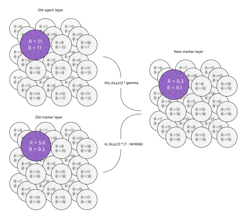
Figure 1 - This figure shows an example of a lattice with L = 3 and D = 3. The example highlights how the markers are updated at position (0,0,0). A new lattice is created to store the next iteration of markers. The old data from the marker and agent layers are read and combined to write to the new layer.
The iteration process continues with each agent randomly selecting one of its neighbours, weighted by the number of markers the neighbours possess. As mentioned before, agents prefer neighbours with lower markers of the opposite species. A pseudo-code implementation for moving the red agents is given in Code 1.
Each iteration ends by removing the old lattices and replacing them with the newer ones. If no errors occur, the iteration count increases.
Program 1. - Naive way of moving the red agents
# Loop over every agent and marker node in the old lattices
Foreach (agent_node, marker_node, index) in old_lattices.iter()

  # Setup a pseudorandom number generator (PRNG). The seed should depend on the
  # index and iteration amount, as well as a global seed provided by the user.
  prng = new PRNG(index, iteration, seed)

  # Get the 6 neighbours of this marker node
  neighbour_markers = marker_node.neighbours()
  blue_strength = [] # Store push strengths of all neighbours

  Foreach marker in neighbour_markers.iter()
    # Append the blue strength for each marker defined in equation
    blue_strengths.push(pow(e, -beta x marker.blue_value))

  # Loop over each red_agent and move it to one of its neighbours
  # according to the strengths of the blue markers
  Foreach red_agent in agent_node.red_agents.iter()
    # Pick one of the neighbours and return the chosen direction to move
    # in (Top, Left, Front, etc.). More info about the method in appendix A.
    direction = PICK_WEIGHTED(prng, blue_strengths)

    # Get the neighbours index from the direction
    new_index = agent_node.index_from_dir(direction)

    # Increment the new lattice with agent nodes at the position of new_index by one
    new_lattices.agent_nodes.add_red_agent(new_index)
3.3. CPU improvements
The straightforward nature of the naive model makes it easy to understand and apply using the mathematics provided. However, as will be shown in Table 1, its execution speed is slow. Iteration is the most time-consuming part of the process. The model is built only once, but the program may have to iterate thousands or even millions of times. To speed up this process while still producing the same output, this section will introduce a faster method of iteration.
Introducing parallel CPU computing can be a good solution when algorithms are running slowly [CCPM14]. Ideally, using K threads can speed up your program by a factor of K. However, this comes with a cost of unpredictability when multiple threads write to the same memory address. This can lead to a behaviour known as a ‘race condition’ [LWZW22].
Race conditions can introduce unpredictable and unstable behaviour. An example can be where an agent is moving from one node to another. When threads A and B read the agent count of node X simultaneously and both try to write one agent to it, only one agent will be added to node X. This results in a loss of total agents which is not allowed in this model. A Mutex prevents simultaneous access to a piece of memory, though this comes with a performance cost as only one thread can access it at a time. By performing all writing calculations within each node and spawning one thread per node, we ensure that only one thread is writing to a memory address during the node’s lifetime.
Only the walking part needs to be updated from the naive model, as updating the markers is not writing to other nodes other than itself, as shown in Figure 1. Code 1 is adopted, whereby each node can read all other nodes but can only write to its own. An impression of how the movement of red agents is changed is visible in Code 2.
Program 2. - Moving red agents with parallisation
new_lattices = new Lattices(old_lattices.parameters)

Foreach (agent_node, marker_node, index) in old_lattices.iter()
  # Move agents out by storing the newly distributed agents in this agent node
  neighbour_markers = marker_node.neighbours()
  prng = new PRNG(index, iteration);
  agents_out = {top:0,right:0,front:0,bottom:0,left:0,back:0}

  Foreach red_agent in agent_node.red_agents.iter()
    # Set of blue strength for each neighbouring node
    blue_strengths = neighbour_markers.blue_strengths
    dir = pick_weighted(prng, blue_strengths)
    agents_out[dir] += 1

  # Write the number of agents that will go to each neighbour to own (index) of the new agent node
  new_lattices.agent_nodes[index].red_agents_out(agents_out)

  Foreach (agent_node, index) in new_lattices.iter()
    # Read agents from neighbouring nodes and move to this node. For instance, get top neighbours agents that should move down (i.e. to this node).
    neighbour_agents = agent_node.neighbours()
    total_red_agents = 0

    Foreach dir in neighbour_agents.iter()
      # Set of all agents in the neighbour at dir (top, right, etc)
      red_agents_dir = neighbour_agents[dir].red_agents_out

      # Add red agents from dir.opposite (top -> bottom, right -> left)
      total_red_agents += red_agents_dir[dir.opposite]

    # Set red agents that this node gets from all neighbours
    agent_node.red_agents(total_red_agents)
3.4. GPU improvements
The speed of the parallelised CPU implementation was still insufficient, as will be discussed in Subsection 4.1. Most GPUs have many more working threads compared to CPUs, this means that GPUs are able to do parallel computations. The GPU implementation was written using WebGPU [MJN23] as the core technology. This web API provides direct access to most GPUs on desktop computers, making the model versatile and more easily reproducible.
WebGPU is often described as a successor of WebGL. WebGL was mostly used for drawing images on the browser screen, whereas WebGPU was designed from the ground up to handle complex GPU computations. WebGPU uses its own shader-language WGSL to reach near-native performance.
GPUs have one downside: data transfers between the CPU and GPU take a relatively significant amount of time. The algorithm is designed to use a ping-pong buffer to store the old and new lattices in GPU memory, reducing the time needed to transfer data to the CPU. A ping-pong buffer consists of two buffers that are used in an alternating fashion. One buffer is used for input, while the other is used for output. Each iteration they swap their function as input or output buffer. This technique reduces latency and enhances performance in real-time applications.
3.5. Visualisations
To interpret the raw data model, several visualisation methods have been developed. These fall into three categories: 2D slice, 3D View and Real-time data view. These categories can be seen in Figure 2. To study these views in detail, visit https://3d-walker.vercel.app/vision/slice for a live view. The purpose for each category is explained further in the respective paragraphs.
The left figure is the slice view and is useful for comparing the current 3D state to the 2D one. If patterns similar to those expected from the 2D case start emerging from a given configuration, it often indicates that we are moving towards an interesting state to compare against. However, each slice is in general an invalid 2D state because agents can cluster and move to slices in the front and back. The assumption of an equal number of agents from species A and B is often not true, so direct comparisons should be made with caution.
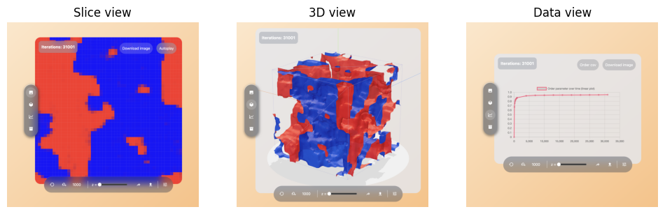
Figure 2 - Left: 2D slicing view. Centre: 3D view and right: data view. All three views display the visuals for lattice area , iterations 31001, , , .
The centre figure shows the 3D view. Drawing each node as a coloured block is difficult to interpret in 3D, because blocks that are hidden by others are hard to spot. The marching cubes algorithm [LC87] is often used in the three-dimensional visualisation of territories. This technique shows the border at which species are equally dominant. Blue-shaded areas describe territories, where the blue species is most dominant. Observe how the slicing view at index z=0 is recognised at the front (left) side of the cube.
Lastly, the right figure is real-time data view. This is for abstracting the visuals away and showing condensed metrics about the model. Here, the order parameter over time which will be defined in Subsection 3.6 is shown. Hovering over each data point reveals the exact order parameter at each time step.
3.6. 3D order parameter
The previous territorial paper employed an order parameter to measure the effect of various parameters on the state of well-mixed versus segregated systems. The order parameter (as defined in Equation 3 is adapted to use agent densities in three dimensions, where the agent density of species i is formulated as (amount of agents at position (x,y,z) and time t) .
Equation 7. - order param 3d
The normalisation coefficient is adapted too. We divide the entire equation by the product of the number of neighbours, lattice area, and total mass squared. This keeps the order parameter bounded at 1, making comparisons between papers easier.
4. Results
Having established the methodology for defining the model with varying levels of complexity, we explain why speed-ups were necessary in Subsection 4.1. These speed-ups enabled us to simulate multiple models and compare them to some properties of the previous territorial paper; using the newly established order parameter. Subsection 4.2 presents how the phase transition is affected by different parameters in our model.
4.1. Compare algorithm speed
The advantage of improving the time-complexity of our model is evident when Table 1 is examined. Parallelisation on a CPU yields approximately five times the speedup of serialisation. Introducing GPU acceleration yields another approximately 200-fold improvement between CPU and GPU parallelization for larger iterations. Table 1 does not take the initialisation step into consideration, because most of the time will be spent in the iteration step, especially with many iterations.
| Iterations | CPU Serial | CPU Parallel | GPU Parallel |
|---|---|---|---|
| 1 | 5.13s | 999ms | 54ms |
| 10 | 40.70s | 9.48s | 99ms |
| 100 | 6m 55s | 1m 37s | 388ms |
| 1000 | 62m 13s | 11m 12s | 2852ms |
Table 1 - Iteration process for the three different methods of computing in Subsection 3.2, Subsection 3.3 and Subsection 3.4. These tests were performed on a Mac-Book Pro with a M1 Pro chip, 12 CPU cores, 14 GPU cores and 32 GB RAM.
The CPU’s speed is approximately ten times slower when performing ten times the work, while the GPU does not follow this pattern. This may be due to the significant time overhead involved in transferring data between the CPU and GPU during GPU computations. Data is transferred from the CPU to GPU when the model is initialised. Measuring the state of the model requires data to be transferred from the GPU to the CPU.
To enhance the algorithm’s speed, it is advisable to minimise the number of measurements taken, as demonstrated in Table 2. Each row displays the number of measures performed for getting to time step 1000, the number of iterations between measurements and the total time taken to reach the 1000 step. The table shows that measuring less will drastically improve the run-time of the algorithm. Often, we only need the final state of the model to compare the 2D and 3D models. We’ll explain this further in Subsubsection 4.2.2.
| Measures | Iterations between | Time |
|---|---|---|
| 1 | 1000 | 2s 852ms |
| 10 | 100 | 3s 313ms |
| 100 | 10 | 6s 85ms |
| 1000 | 1 | 46s 449ms |
Table 2 - Iterating to P iterations can be done with M measurements where M spans 0 to P in between P/M iterations. Doing fewer measurements between iterations will speed up the GPU algorithm significantly. For this table, the value 1000 is used for P.
4.2. Comparing phase transitions between papers
Previous research showed that various parameters had a significant impact on the phase transition of the model. We first detect a phase transition in our model in Subsubsection 4.2.1. Then, we analyse how total mass affects both 2D and 3D models in Subsubsection 4.2.2. Finally, we compare phase transition with the ratio of between models in Subsubsection 4.2.3.
4.2.1. Well-mixed, well-segregated and partial-segregated states
The random walker model from A. Alsenafi and A.B. Barbaro [AB18] identified three different states for a model.
- Well-mixed: Species will move with an unbiased walk. This is translated to a low beta value.
- Partial-segregated: Species will move together, but not to the point of complete separation.
- Well-segregated: Species will move to a state where only two territories remain, one for each species. This corresponds to a beta parameter approaching 1.
These states were also observed for the 3D model. This can be observed in Figure 3, where all images are using , the total mass is 12.5 million (50 agents per node per species) and an iteration count of 60,000. The top left image is a state observed at iteration 0. Because each agent starts off at a uniformly random location, this state is by definition a well-mixed state. The top right image displays a mix of blue and red species with many small territories. This suggests that species do not form distinct territories and remain well-mixed. The bottom left image depicts a partially segregated state with some islands of territories. We can see that agents have formed some structures from the initially mixed state, making them partially segregated. The bottom right image is well-segregated, with large territories for each species.
Understanding how the model would further evolve can be done by looking at the trend of the order parameter defined in Equation 7. The corresponding order parameters over time for Figure 3 are displayed in Figure 4. All states reach 90% of their final order parameter before 1000 iterations. At the 20000 iteration mark, all states have reached over 97% of their final order parameter. We notice from the evolution of the order parameter that the segregation occurs well before the first 50000 iterations.
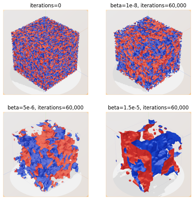
Figure 3 - Top left: A model without iterating over it, all models start off as well-mixed. Top right: A model with beta = 1e-8, this model is still classified as well-mixed. Bottom left: A model with beta = 5e-6, this model is classified as partial-segregated. Bottom right: A model with beta 1.5e-5, and is classified as well-segregated. All models have total mass of 12.5 million, lattice area = and .
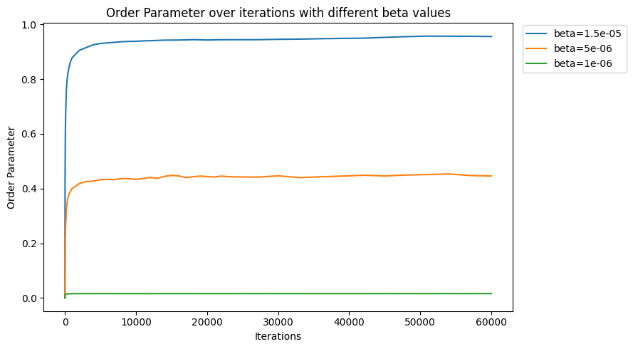
Figure 4 - Order parameters for different beta values corresponding to (from top to bottom) a well-segregated, partial-segregated and well-mixed state. Using a lattice length of 50, the mass is 12.5 million, and .
4.2.2. Comparing mass parameters
Using the knowledge from Subsubsection 4.2.1, the model is unlikely to switch from well-mixed to well-segregated after 50,000 iterations. The previous territory paper concluded that using more mass corresponds to fewer beta required to reach a segregated state.
After 50,000 iterations, we calculate the final order parameter value for three different beta values. The results are presented in Figure 5. We set the critical to be the same as the previous paper for easier comparison. This corresponds to an order parameter of 0.01, which we denote as . Validation that this value is correct in 3D is provided in Appendix B.
The first plot in Figure 5 shows that for a mass of 1,600,000, the critical value for the phase transition is approximately . In contrast, when the mass is increased to 3,200,000, the critical value decreases to around , as shown in the right plot. These findings suggest that as the system’s mass increases, the critical value for the phase transition decreases. This observation is consistent with the previous work on 2D territory formation.
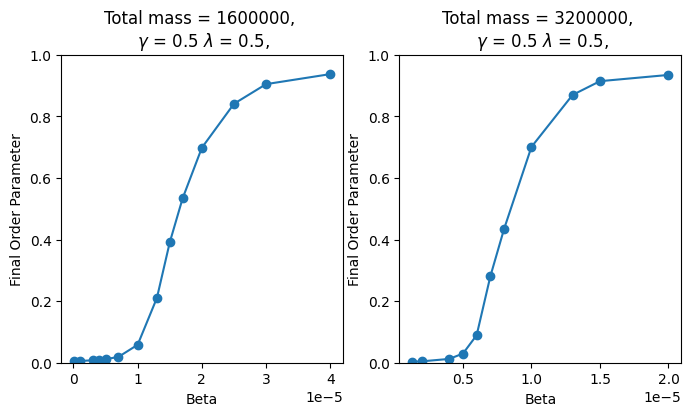
Figure 5 - Final order-parameters for different values of beta. The left graph has a total mass of 1,600,000, and the right has a total mass of 3,200,000. Both graphs were produced with a lattice length of 20, and .
Generalising this finding with different masses to critical betas is shown in Figure 6. The continuous stability analysis is plotted next to our measurements. It can be observed how the discrete 3D model has a similar shape to the two-dimensional stability analysis case.
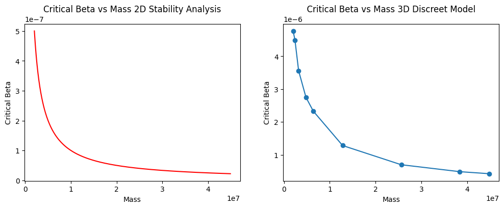
Figure 6 - Critical for different total masses. Left: (their) 2D stability analysis, measure where taken with lattice length of 50, and . Right: (our) 3D discreet model, measures were taken with a lattice length of 20, and .
4.2.3. Comparing lambda/gamma parameters
The same procedure can be done to compare the behaviour of the ratio of gamma and lambda. The previous paper concluded that changing and making the ratio of gamma/lambda smaller resulted in an approximate doubling of critical beta.
We investigated this finding in three dimensions for two ratios: 0.25/0.5 and 0.75/0.5 (see Figure 7). The ratio of 1/2 was measured with a critical beta of 7.14e-6. When the ratio was increased to 3/2, the critical beta decreased to 2.27e-6. This roughly corresponds to a threefold decrease in critical beta. This finding is consistent with previous research on two-dimensional territory formation.
Figure 8 reveals generalised measurements for a range of ratios. We plot our 3D model findings alongside the previous 2D model results. We scale both axes to the same size to allow for better analysis. The graphs have a similar shape, although remember that the total mass and lattice sizes differ between models.
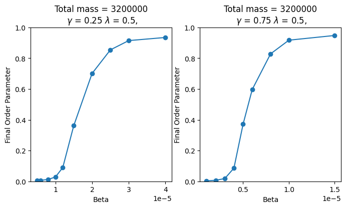
Figure 7 - Final order-parameters for different ratios of . The left graph has a ratio of 0.25/0.5 = 1/2, and the right has a ratio of 0.75/0.5 = 3/2. Both graphs were produced with a lattice length of 20, and a total mass of 3,200,000.
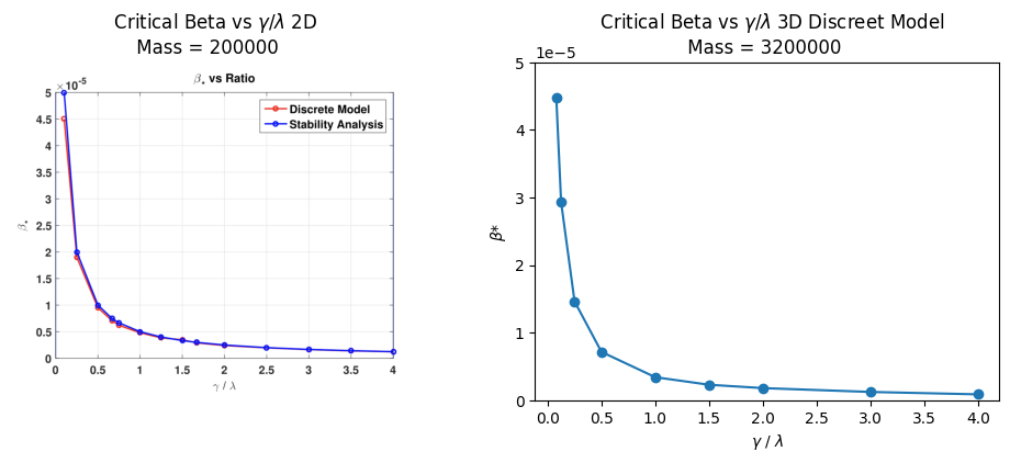
Figure 8 - Critical for different ratios of . Left: (their) 2D analysis both stability analysis and discrete measurements, measures were taken with a lattice length of 50, total mass = 200,000. Right: (our) 3D discreet model, measures were taken with a lattice length of 20, and a total mass of 3,200,000.
5. Argumentation and discussion
Using the results obtained in the previous section, we address the limitations of the presented model for territory formation, which includes the consideration of how well our comparisons can be made between models. However, the section will also explore the possibilities for future work, such as the extension of the model to multiple species, the exploration of different metrics for analysing behavioural patterns, and the application of the model to other fields of research, such as disease spread.
5.1. Discuss results
This section revisits the two sub-questions asked in the introduction to determine if they have been adequately answered. Each sub-question is elaborated in its own subsection.
5.1.1. Three-dimensional lattice phase states
The first sub-question to be discussed is: “What are the states of the three-dimensional lattice model, and are they well-mixed or well-segregated”. Well-mixed states are, by definition, present at the start of each model. Figure 3 and Figure 4 demonstrate how an ordered state is created from chaos. We observed that larger values of beta produce larger territories, which are classified as well-segregated.
The previous paper noted that models showed signs of segregation after the order parameter surpassed the value of 0.01. The same threshold was chosen for our model for better comparisons. Curious readers can find multiple two-dimensional slices and three-dimensional models in the Appendix validation, which validate that the threshold is still a valid measure.
5.1.2. Contrast and similarities between models
The second sub-question was: “How does mass and gamma/lambda ratio influence the phase transition of the 3D model?”. Figure 5 and Figure 7 demonstrate that similarly to the findings of the previous paper, increasing the total mass or the to ratio decreases the amount of beta required to reach a segregated state.
To determine if the behaviour was consistent across a wider range of masses and ratios, we plotted them and compared them to the 2D model. We noticed that the graph shape was similar between the models, concluding that the same behaviour could be observed. We take caution when making direct comparisons between models; this will be discussed in Subsection 5.2.
5.2. Discussion on discreet models
Analysis of the critical beta parameter in relation to total mass for both 2D continuous and 3D discrete models displays similar behaviour across dimensions. However, a noteworthy difference is that the 3D model needs significantly more beta to reach the same critical point for each total mass. The same holds for comparing the behaviour of ratio.
The main cause for this large increase must be linked to the number of dimensions an agent can walk towards. Other smaller factors may also be involved. To enable direct comparisons between models, a continuous 3D model should be developed for further analysis.
Discrete models are useful for exploring new behaviours, while continuous models provide more accurate representations for comparing models. Continuous models eliminate random fluctuations that can be introduced by discrete models. In summary, further research should be devoted to transforming our discrete results into a continuous model to allow for direct comparisons between models.
5.3. Find other metrics
Research is a collaborative effort, and often, one study can lead to the discovery of new insights and avenues for exploration. Because this paper has an accessible web version published, it is easy to find new interesting behaviour for other researchers.
In the background of this paper, in Subsection 2.1 it is noted that the amount of data that can be generated with random walker models is endless. An infinite amount of parameters and iterations can be combined to produce a meaningful output. This paper computes behavioural patterns using our order parameter, defined in Subsection 3.6. Different (order) functions can be defined to analyse different types of behavioural patterns in territory formation.
For example, M. Skrodzki et al. [SRZ21] uncovered a metric related to the typology of certain states in three-dimensional Turing-like patterns. Further research can be conducted into finding a similar behaviour for our three-dimensional patterns .
In their extension paper [AB21], A. Alsenafi and A.B. Barbaro proposed a multi-species model (with n>2) that has many new intriguing properties relevant to this paper. Examining how the many species would interact with one another could provide meaningful insight into the realm of micro-organisms.
5.4. Other fields of research
This paper was inspired by micro-organisms forming a territory. However, this paper is mathematically created so it can be extended to many other fields of research.
Territory formation is also apparent for ant colony formation [L21] [T11]. Ants are known for their remarkable ability to form complex societies, which are often characterised by the formation of territories. These territories are established through a variety of mechanisms, including chemical communication. However, studying ant behaviour in the wild can be challenging due to the harsh environments in which they live and the confined spaces in which they operate. By using computer models, researchers can manipulate various parameters and observe how they affect ant colony behaviour, allowing them to gain insights into the underlying mechanisms of ant colony formation.
6. Conclusion
We conclude that the main question: “What similarities exist between properties of the two-dimensional and three-dimensional lattice models?” can be answered by that both models have a well-mixed and segregated state. Furthermore, the point at which the state changes from well-mixed to well-segregated is in both models determined by the amount of mass present in the lattices and the ratio between plays a large role. For both models, the more mass or they have, the less beta is required to reach the critical point. Additionally, the 3D model needs significantly more beta to reach the same critical point for the same amount of mass or ratio.
We conclude that the model has many behaviours that remain unexplored in this paper. Making the model easily accessible to other researchers can enable the measurement and observation of more interesting behaviours, helping to better understand the complex world of higher-dimensional random walks.
Bibliography
7. Responsible research
Responsibility in research was carefully considered while writing this paper. All images referenced in this paper are easy to reproduce with the public web app created alongside this paper. The code for this paper is available on GitHub ( https://github.com/yustarandomname/territories-in-three-dimensions) under the MIT license, allowing abundant opportunities for extension. The code is thus reproducible and extendable for future work. Finally, any work used by other researchers is properly cited and referenced in the text to locate the sources correctly.
We were supplied with the original code from the previous territory paper. However, this code was not reproducible on the machines used by the author. Our method was created from scratch and checked with the mathematics from the paper. Small discrepancies could be the result of this method. For instance, differences in PRNGs (Pseudo Random Number Generators) could give small differences between results. We thus opted to look if the behaviour between models was similar and were careful with making direct comparisons between models. We noted that direct comparisons are only possible if our method was reproduced with a continuous mathematical model.
Finally, the author listed on the title page wrote the entire original paper. AI models like OpenAI GPT-4 and Grammarly were used to enhance grammar and readability. The author and several others validated all the changes.